Category: <span>Announcements</span>

AWS Machine Learning University New Educator Enablement Program to Build Diverse Talent for ML/AI Jobs

AWS Machine Learning University is now providing a free educator enablement program. This program provides faculty at community colleges, minority-serving institutions (MSIs), and historically Black colleges and universities (HBCUs) with the skills and resources to teach data analytics, artificial intelligence (AI), and machine learning (ML) concepts to build a diverse pipeline for in-demand jobs of today and tomorrow.

According to the National Science Foundation, Black and Hispanic or Latino students earn bachelor’s degrees in Computer Science—the dominant pathway to AI/ML—at a much lower rate than their white peers, earning less than 11 percent of computer science degrees awarded. However, research shows that having diverse perspectives among skilled practitioners and across the AI/ML lifecycle contributes to the development of AI/ML systems that are safe, trustworthy, and have less bias. 

In 2018, we announced the Machine Learning University (MLU) to share with all developers the same courses that we used to train engineers at Amazon and AWS. This platform offers self-service, self-paced, AI/ML digital courses.

Machine Learning University home page

And today, we add this new program to our AI/ML training offering. Although anyone could access the MLU self-paced learning, it places the burden on the learner to source prerequisite work and solutions. This educator enablement program takes the concepts and lessons developed by MLU and makes them more accessible to educators. It offers a year-round educator enablement program with lesson planning, course playbooks, and access to free compute resources.

Program Details
Educators are onboarded in small-group cohorts into bootcamps where they will learn the material and deep dive into how to teach it via instructor-led lectures and hands-on projects. Educators who complete the bootcamp can take part in different year-round development opportunities, such as a dedicated Slack channel to share teaching best practices, education topic series and virtual study sessions moderated by MLU instructors, and regional events for continued professional development. Also, they will receive continuing education credits and AWS-provided stipends.

Faculty and students get access to instructional material through Amazon SageMaker Studio Lab. SageMaker Studio Lab was announced last year and is AWS’s free (no credit card required) ML development environment. It provides computing and storage for anybody that wants to learn and experiment with ML. Institutions can unlock additional resources to support their ML programs by registering for AWS Academy. AWS Academy unlocks all the AWS services for a complete AI/ML program.

Community colleges and universities can integrate this educator enablement program into their computer science, information technology, and business curricula to create an AI/ML course, certificate, or degree. We have worked with educators and education boards such as Houston Community College to create content that is vetted for credit-worthy and degree-earning curricula.

In August 2022, we launched our first educator bootcamp in partnership with The Coding School. The bootcamp was delivered over two weeks, offering lectures, case studies, and hands-on projects. 25 educators completed the Educator Machine Learning Bootcamp, representing 22 US community colleges and universities.

Learn More and Join The Program
During 2023, AWS Machine Learning University will run six educator-enablement cohorts starting in January. The program will give priority consideration to educators at community colleges, MSIs, and HBCUs, in alignment with this program mission to increase access to AI/ML technology to historically underserved and underrepresented students.

If you are a computer science educator or part of a board of educators interested in fostering more depth in your computer science coursework, you should sign up for the educator enablement program.

Marcia

New for Amazon Redshift – Simplify Data Ingestion and Make Your Data Warehouse More Secure and Reliable

When we talk with customers, we hear that they want to be able to harness insights from data in order to make timely, impactful, and actionable business decisions. A common pattern with data-driven organizations is that they have many different data sources they need to ingest into their analytics systems. This requires them to build manual data pipelines spanning across their operational databases, data lakes, streaming data, and data within their warehouse. As a consequence of this complex setup, it can take data engineers weeks or even months to build data ingestion pipelines. These data pipelines are costly, and the delays can lead to missed business opportunities. Additionally, data warehouses are increasingly becoming mission critical systems that require high availability, reliability, and security.

Amazon Redshift is a fully managed petabyte-scale data warehouse used by tens of thousands of customers to easily, quickly, securely, and cost-effectively analyze all their data at any scale. This year at re:Invent, Amazon Redshift has announced a number of features to help you simplify data ingestion and get to insights easily and quickly, within a secure, reliable environment.

In this blog, I introduce some of these new features that fit into two main categories:

  • Simplify data ingestion
    • Amazon Redshift now supports auto-copy from Amazon S3 (available in preview). With this new capability, Amazon Redshift automatically loads the files that arrive in an Amazon Simple Storage Service (Amazon S3) location that you specify into your data warehouse. The files can use any of the formats supported by the Amazon Redshift copy command, such as CSV, JSON, Parquet, and Avro. In this way, you don’t need to manually or repeatedly run copy procedures. Amazon Redshift automates file ingestion and takes care of data-loading steps under the hood.
    • With Amazon Aurora zero-ETL integration with Amazon Redshift, you can use Amazon Redshift for near real-time analytics and machine learning on petabytes of transactional data stored on Amazon Aurora MySQL databases (available in limited preview). With this capability, you can choose the Amazon Aurora databases containing the data you want to analyze with Amazon Redshift. Data is then replicated into your data warehouse within seconds after transactional data is written into Amazon Aurora, eliminating the need to build and maintain complex data pipelines. You can replicate data from multiple Amazon Aurora databases into the same Amazon Redshift instance to run analytics across multiple applications. With near real-time access to transactional data, you can leverage Amazon Redshift’s analytics and capabilities, such as built-in machine learning (ML), materialized views, data sharing, and federated access to multiple data stores and data lakes, to derive insights from transactional and other data.
    • With the general availability of Amazon Redshift Streaming Ingestion, you can now natively ingest hundreds of megabytes of data per second from Amazon Kinesis Data Streams and Amazon MSK into an Amazon Redshift materialized view and query it in seconds. Learn more in this post.
  • Make your data warehouse more secure and reliable
    • You can now improve the availability of your data warehouse by choosing multiple Availability Zone (AZ) deployments. Multi-AZ deployments for your Amazon Redshift clusters are available in preview and reduce recovery times to seconds through automatic recovery. In this way, you can build solutions that are more compliant with the recommendations of the Reliability Pillar of the AWS Well-Architected Framework.
    • With dynamic data masking (available in preview), you can protect sensitive information stored in your data warehouse and ensure that only the relevant data is accessible by users based on their roles. You can limit how much identifiable data is visible to users using multiple levels of policies so different users and groups can have different levels of data access without having to create multiple copies of data. Dynamic data masking complements other granular access control capabilities in Amazon Redshift including row-level and column-level security and role-based access controls. In this way, Dynamic Data Masking helps you meet requirements for GDPR, CCPA, and other privacy regulations.
    • Amazon Redshift now supports central access controls for data sharing with AWS Lake Formation (available in public preview). You can now use Lake Formation to simplify governance of data shared from Amazon Redshift and centrally manage granular access across all data-sharing consumers.

There have been other interesting news for Amazon Redshift at re:Invent you might have already heard about:

  • The general availability of Amazon Redshift integration for Apache Spark makes it easy to build and run Spark applications on Amazon Redshift and Redshift Serverless, opening up the data warehouse for a broader set of AWS analytics and machine learning solutions.
  • AWS Backup now supports Amazon Redshift. AWS Backup allows you to define a central backup policy to manage data protection of your applications and can also protect your Amazon Redshift clusters. In this way, you have a consistent experience when managing data protection across all supported services.

Availability and Pricing
Multi-AZ deployments, central access control for data sharing with AWS Lake Formation, auto-copy from Amazon S3, and dynamic data masking are available in preview in US East (Ohio), US East (N. Virginia), US West (Oregon), Asia Pacific (Tokyo), Europe (Ireland), and Europe (Stockholm).

There is no additional cost for using auto-copy from Amazon S3 and near real-time analytics on transactional data. There is no extra charge for dynamic data masking and central access control for data sharing. For more information, see Amazon Redshift pricing.

These new capabilities take you one step further in analyzing all your data across data sources with simple data ingestion capabilities, while improving the security and reliability of your data warehouse.

Danilo

New — Introducing Support for Real-Time and Batch Inference in Amazon SageMaker Data Wrangler

To build machine learning models, machine learning engineers need to develop a data transformation pipeline to prepare the data. The process of designing this pipeline is time-consuming and requires a cross-team collaboration between machine learning engineers, data engineers, and data scientists to implement the data preparation pipeline into a production environment.

The main objective of Amazon SageMaker Data Wrangler is to make it easy to do data preparation and data processing workloads. With SageMaker Data Wrangler, customers can simplify the process of data preparation and all of the necessary steps of data preparation workflow on a single visual interface. SageMaker Data Wrangler reduces the time to rapidly prototype and deploy data processing workloads to production, so customers can easily integrate with MLOps production environments.

However, the transformations applied to the customer data for model training need to be applied to new data during real-time inference. Without support for SageMaker Data Wrangler in a real-time inference endpoint, customers need to write code to replicate the transformations from their flow in a preprocessing script.

Introducing Support for Real-Time and Batch Inference in Amazon SageMaker Data Wrangler
I’m pleased to share that you can now deploy data preparation flows from SageMaker Data Wrangler for real-time and batch inference. This feature allows you to reuse the data transformation flow which you created in SageMaker Data Wrangler as a step in Amazon SageMaker inference pipelines.

SageMaker Data Wrangler support for real-time and batch inference speeds up your production deployment because there is no need to repeat the implementation of the data transformation flow. You can now integrate SageMaker Data Wrangler with SageMaker inference. The same data transformation flows created with the easy-to-use, point-and-click interface of SageMaker Data Wrangler, containing operations such as Principal Component Analysis and one-hot encoding, will be used to process your data during inference. This means that you don’t have to rebuild the data pipeline for a real-time and batch inference application, and you can get to production faster.

Get Started with Real-Time and Batch Inference
Let’s see how to use the deployment supports of SageMaker Data Wrangler. In this scenario, I have a flow inside SageMaker Data Wrangler. What I need to do is to integrate this flow into real-time and batch inference using the SageMaker inference pipeline.

First, I will apply some transformations to the dataset to prepare it for training.

I add one-hot encoding on the categorical columns to create new features.

Then, I drop any remaining string columns that cannot be used during training.

My resulting flow now has these two transform steps in it.

After I’m satisfied with the steps I have added, I can expand the Export to menu, and I have the option to export to SageMaker Inference Pipeline (via Jupyter Notebook).

I select Export to SageMaker Inference Pipeline, and SageMaker Data Wrangler will prepare a fully customized Jupyter notebook to integrate the SageMaker Data Wrangler flow with inference. This generated Jupyter notebook performs a few important actions. First, define data processing and model training steps in a SageMaker pipeline. The next step is to run the pipeline to process my data with Data Wrangler and use the processed data to train a model that will be used to generate real-time predictions. Then, deploy my Data Wrangler flow and trained model to a real-time endpoint as an inference pipeline. Last, invoke my endpoint to make a prediction.

This feature uses Amazon SageMaker Autopilot, which makes it easy for me to build ML models. I just need to provide the transformed dataset which is the output of the SageMaker Data Wrangler step and select the target column to predict. The rest will be handled by Amazon SageMaker Autopilot to explore various solutions to find the best model.

Using AutoML as a training step from SageMaker Autopilot is enabled by default in the notebook with the use_automl_step variable. When using the AutoML step, I need to define the value of target_attribute_name, which is the column of my data I want to predict during inference. Alternatively, I can set use_automl_step to False if I want to use the XGBoost algorithm to train a model instead.

On the other hand, if I would like to instead use a model I trained outside of this notebook, then I can skip directly to the Create SageMaker Inference Pipeline section of the notebook. Here, I would need to set the value of the byo_model variable to True. I also need to provide the value of algo_model_uri, which is the Amazon Simple Storage Service (Amazon S3) URI where my model is located. When training a model with the notebook, these values will be auto-populated.

In addition, this feature also saves a tarball inside the data_wrangler_inference_flows folder on my SageMaker Studio instance. This file is a modified version of the SageMaker Data Wrangler flow, containing the data transformation steps to be applied at the time of inference. It will be uploaded to S3 from the notebook so that it can be used to create a SageMaker Data Wrangler preprocessing step in the inference pipeline.

The next step is that this notebook will create two SageMaker model objects. The first object model is the SageMaker Data Wrangler model object with the variable data_wrangler_model, and the second is the model object for the algorithm, with the variable algo_model. Object data_wrangler_model will be used to provide input in the form of data that has been processed into algo_model for prediction.

The final step inside this notebook is to create a SageMaker inference pipeline model, and deploy it to an endpoint.

Once the deployment is complete, I will get an inference endpoint that I can use for prediction. With this feature, the inference pipeline uses the SageMaker Data Wrangler flow to transform the data from your inference request into a format that the trained model can use.

In the next section, I can run individual notebook cells in Make a Sample Inference Request. This is helpful if I need to do a quick check to see if the endpoint is working by invoking the endpoint with a single data point from my unprocessed data. Data Wrangler automatically places this data point into the notebook, so I don’t have to provide one manually.

Things to Know
Enhanced Apache Spark configuration — In this release of SageMaker Data Wrangler, you can now easily configure how Apache Spark partitions the output of your SageMaker Data Wrangler jobs when saving data to Amazon S3. When adding a destination node, you can set the number of partitions, corresponding to the number of files that will be written to Amazon S3, and you can specify column names to partition by, to write records with different values of those columns to different subdirectories in Amazon S3. Moreover, you can also define the configuration in the provided notebook.

You can also define memory configurations for SageMaker Data Wrangler processing jobs as part of the Create job workflow. You will find similar configuration as part of your notebook.

Availability — SageMaker Data Wrangler supports for real-time and batch inference as well as enhanced Apache Spark configuration for data processing workloads are generally available in all AWS Regions that Data Wrangler currently supports.

To get started with Amazon SageMaker Data Wrangler supports for real-time and batch inference deployment, visit AWS documentation.

Happy building
— Donnie

Announcing Additional Data Connectors for Amazon AppFlow

Gathering insights from data is a more effective process if that data isn’t fragmented across multiple systems and data stores, whether on premises or in the cloud. Amazon AppFlow provides bidirectional data integration between on-premises systems and applications, SaaS applications, and AWS services. It helps customers break down data silos using a low- or no-code, cost-effective solution that’s easy to reconfigure in minutes as business needs change.

Today, we’re pleased to announce the addition of 22 new data connectors for Amazon AppFlow, including:

  • Marketing connectors (e.g., Facebook Ads, Google Ads, Instagram Ads, LinkedIn Ads).
  • Connectors for customer service and engagement (e.g., MailChimp, Sendgrid, Zendesk Sell or Chat, and more).
  • Business operations (Stripe, QuickBooks Online, and GitHub).

In total, Amazon AppFlow now supports over 50 integrations with various different SaaS applications and AWS services. This growing set of connectors can be combined to enable you to achieve 360 visibility across the data your organization generates. For instance, you could combine CRM (Salesforce), e-commerce (Stripe), and customer service (ServiceNow, Zendesk) data to build integrated analytics and predictive modeling that can guide your next best offer decisions and more. Using web (Google Analytics v4) and social surfaces (Facebook Ads, Instagram Ads) allows you to build comprehensive reporting for your marketing investments, helping you understand how customers are engaging with your brand. Or, sync ERP data (SAP S/4HANA) with custom order management applications running on AWS. For more information on the current range of connectors and integrations, visit the Amazon AppFlow integrations page.

Datasource connectors for Amazon AppFlow

Amazon AppFlow and AWS Glue Data Catalog
Amazon AppFlow has also recently announced integration with the AWS Glue Data Catalog to automate the preparation and registration of your SaaS data into the AWS Glue Data Catalog. Previously, customers using Amazon AppFlow to store data from supported SaaS applications into Amazon Simple Storage Service (Amazon S3) had to manually create and run AWS Glue Crawlers to make their data available to other AWS services such as Amazon Athena, Amazon SageMaker, or Amazon QuickSight. With this new integration, you can populate AWS Glue Data Catalog with a few clicks directly from the Amazon AppFlow configuration without the need to run any crawlers.

To simplify data preparation and improve query performance when using analytics engines such as Amazon Athena, Amazon AppFlow also now enables you to organize your data into partitioned folders in Amazon S3. Amazon AppFlow also automates the aggregation of records into files that are optimized to the size you specify. This increases performance by reducing processing overhead and improving parallelism.

You can find more information on the AWS Glue Data Catalog integration in the recent What’s New post.

Getting Started with Amazon AppFlow
Visit the Amazon AppFlow product page to learn more about the service and view all the available integrations. To help you get started, there’s also a variety of videos and demos available and some sample integrations available on GitHub. And finally, should you need a custom integration, try the Amazon AppFlow Connector SDK, detailed in the Amazon AppFlow documentation. The SDK enables you to build your own connectors to securely transfer data between your custom endpoint, application, or other cloud service to and from Amazon AppFlow‘s library of managed SaaS and AWS connectors.

— Steve

Amazon Location Service Is Now Generally Available with New Routing and Satellite Imagery Capabilities

In December of 2020, we made Amazon Location Service available in preview form for you to start building web and mobile applications with location-based features. Today I’m pleased to announce that we are making Amazon Location generally available along with two new features: routing and satellite imagery.

I have been a full-stack developer for over 15 years. On multiple occasions, I was tasked with creating location-based applications. The biggest challenges I faced when I worked with location providers were integrating the applications into the existing application backend and frontend and keeping the data shared with the location provider secure. When Amazon Location was made available in preview last year, I was so excited. This service makes it possible to build location-based applications with a native integration with AWS services. It uses trusted location providers like Esri and HERE and customers remain in control of their data.

Amazon Location includes the following features:

  • Maps to visualize location information.
  • Places to enable your application to offer point-of-interest search functionality, convert addresses into geographic coordinates in latitude and longitude (geocoding), and convert a coordinate into a street address (reverse geocoding).
  • Routes to use driving distance, directions, and estimated arrival time in your application.
  • Trackers to allow you to retrieve the current and historical location of the devices running your tracking-enabled application.
  • Geofences to give your application the ability to detect and act when a tracked device enters or exits a geographical boundary you define as a geofence. When a breach of the geofence is detected, Amazon Location will send an event to Amazon EventBridge, which can trigger a downstream set of actions, like invoking an AWS Lambda function or sending a notification using Amazon Simple Notification Service (SNS). This level of integration with AWS services is one of the most powerful features of Amazon Location. It will help shorten your application’s time to production.

In the preview announcement blog post, Jeff introduced the service functionality in a lot of detail. In this blog post, I want to focus on the new two features: satellite imagery and routing.

Satellite Imagery

You can use satellite imagery to pack your maps with information and provide more context to the map users. It helps the map users answer questions like “Is there a swamp in that area?” or “What does that building look like?”

To get started with satellite imagery maps, go to the Amazon Location console. On Create a new map, choose Esri Imagery. 

Creating a new map with satellite imagery

Routing
With Amazon Location Routes, your application can request the travel time, distance, and all directions between two locations. This makes it possible for your application users to obtain accurate travel-time estimates based on live road and traffic information.

If you provide these extra attributes when you use the route feature, you can get very tailored information including:

  • Waypoints: You can provide a list of ordered intermediate positions to be reached on the route. You can have up to 25 stopover points including the departure and destination.
  • Departure time: When you specify the departure time for this route, you will receive a result optimized for the traffic conditions at that time.
  • Travel mode: The mode of travel you specify affects the speed and the road compatibility. Not all vehicles can travel on all roads. The available travel modes are car, truck and walking. Depending on which travel mode you select, there are parameters that you can tune. For example, for car and truck, you can specify if you want a route without ferries or tolls. But the most interesting results are when you choose the truck travel mode. You can define the truck dimensions and weight and then get a route that is optimized for these parameters. No more trucks stuck under bridges!

Amazon Location Service and its features can be used for interesting use cases with low effort. For example, delivery companies using Amazon Location can optimize the order of the deliveries, monitor the position of the delivery vehicles, and inform the customers when the vehicle is arriving. Amazon Location can be also used to route medical vehicles to optimize the routing of patients or medical supplies. Logistic companies can use the service to optimize their supply chain by monitoring all the delivery vehicles.

To use the route feature, start by creating a route calculator. In the Amazon Location console, choose Route calculators. For the provider of the route information, choose Esri or HERE.

Screenshot of create a new routing calculator

You can use the route calculator from the AWS SDKs, AWS Command Line Interface (CLI) or the Amazon Location HTTP API.

For example, to calculate a simple route between departure and destination positions using the CLI, you can write something like this:

aws location 
    calculate-route 
        --calculator-name MyExampleCalculator 
        --departure-position -123.1376951951309 49.234371474778385 
        --destination-position -122.83301379875074 49.235860182576886

The departure-position and destination-positions are defined as longitude, latitude.

This calculation returns a lot of information. Because you didn’t define the travel mode, the service assumes that you are using a car. You can see the total distance of the route (in this case, 29 kilometers). You can change the distance unit when you do the calculation. The service also returns the duration of the trip (in this case, 29 minutes). Because you didn’t define when to depart, Amazon Location will assume that you want to travel when there is the least amount of traffic.

{
    "Legs": [{
        "Distance": 26.549,
        "DurationSeconds": 1711,
        "StartPosition":[-123.1377012, 49.2342994],
        "EndPosition": [-122.833014,49.23592],
        "Steps": [{
            "Distance":0.7,
            "DurationSeconds":52,
            "EndPosition":[-123.1281,49.23395],
            "GeometryOffset":0,
            "StartPosition":[-123.137701,49.234299]},
            ...
        ]
    }],
    "Summary": {
        "DataSource": "Esri",
        "Distance": 29.915115551209176,
        "DistanceUnit": "Kilometers",
        "DurationSeconds": 2275.5813682980006,
        "RouteBBox": [
            -123.13769762299995,
            49.23068000000006,
            -122.83301399999999,
            49.258440000000064
        ]
    }
}

It will return an array of steps, which form the directions to get from departure to destination. The steps are represented by a starting position and end position. In this example, there are 11 steps and the travel mode is a car.

Screenshot of route drawn in map

The result changes depending on the travel mode you selected. For example, if you do the calculation for the same departure and destination positions but choose a travel mode of walking, you will get a series of steps that draw the map as shown below. The travel time and distance are different: 24.1 kilometers and 6 hours and 43 minutes.

Map of route when walking

Available Now
Amazon Location Service is now available in the US East (N. Virginia), US East (Ohio), US West (Oregon), Europe (Frankfurt), Europe (Ireland), Europe (Stockholm), Asia Pacific (Singapore), Asia Pacific (Sydney), and Asia Pacific (Tokyo) Regions.

Learn about the pricing models of Amazon Location Service. For more about the service, see Amazon Location Service

Marcia

In the Works – AWS Region in the United Arab Emirates (UAE)

We are currently building AWS regions in Australia, Indonesia, Spain, India, and Switzerland.

UAE in the Works
I am happy to announce that the AWS Middle East (UAE) Region is in the works and will open in the first half of 2022. The new region is an extension of our existing investment, which already includes two AWS Direct Connect locations and two Amazon CloudFront edge locations, all of which have been in place since 2018. The new region will give AWS customers in the UAE the ability to run workloads and to store data that must remain in-country, in addition to the ability to serve local customers with even lower latency.

The new region will have three Availability Zones, and will be the second AWS Region in the Middle East, joining the existing AWS Region in Bahrain. There are 80 Availability Zones within 25 AWS Regions in operation today, with 15 more Availability Zones and five announced regions underway in the locations that I listed earlier.

As is always the case with an AWS Region, each of the Availability Zones will be a fully isolated part of the AWS infrastructure. The AZs in this region will be connected together via high-bandwidth, low-latency network connections to support applications that need synchronous replication between AZs for availability or redundancy.

AWS in the UAE
In addition to the upcoming AWS Region and the Direct Connect and CloudFront edge locations, we continue to build our team of account managers, partner managers, data center technicians, systems engineers, solutions architects, professional service providers, and more (check out our current positions).

We also plan to continue our on-going investments in education initiatives, training, and start-up enablement to support the UAE’s plans for economic development and digital transformation.

Our customers in the UAE are already using AWS to drive innovation! For example:

Mohammed Bin Rashid Space Centre (MBRSC) – Founded in 2006, MBSRC is home to the UAE’s National Space Program. The Hope Probe was launched last year and reached Mars in February of this year. Data from the probe’s instruments is processed and analyzed on AWS, and made available to the global scientific community in less than 20 minutes.

Anghami is the leading music platform in the Middle East and North Africa, giving over 70 million users access to 57 million songs. They have been hosting their infrastructure on AWS since their days as a tiny startup,. and have benefited from the ability to scale up by as much as 300% when new music is launched.

Sarwa is an investment bank and personal finance platform that was born on the AWS cloud in 2017. They grew by a factor of four in 2020 while processing hundreds of thousands of transactions. Recent AWS-powered innovations from Sarwa include the Sarwa App (design to market in 3 months) and the upcoming Sarwa Trade platform.

Stay Tuned
We’ll be announcing the opening of the Middle East (UAE) Region in a forthcoming blog post, so be sure to stay tuned!

Jeff;

New – AWS App Runner: From Code to a Scalable, Secure Web Application in Minutes

Containers have become the default way that I package my web applications. Although I love the speed, productivity, and consistency that containers provide, there is one aspect of the container development workflow that I do not like: the lengthy routine I go through when I deploy a container image for the first time.

You might recognize this routine: setting up a load balancer, configuring the domain, setting up TLS, creating a CI/CD pipeline, and deploying to a container service.

Over the years, I have tweaked my workflow and I now have a boilerplate AWS Cloud Development Kit project that I use, but it has taken me a long time to get to this stage. Although this boilerplate project is great for larger applications, it does feel like a lot of work when all I want to do is deploy and scale a single container image.

At AWS, we have a number of services that provide granular control over your containerized application, but many customers have asked if AWS can handle the configuration and operations of their container environments. They simply want to point to their existing code or container repository and have their application run and scale in the cloud without having to configure and manage infrastructure services.

Because customers asked us to create something simpler, our engineers have been hard at work creating a new service you are going to love.

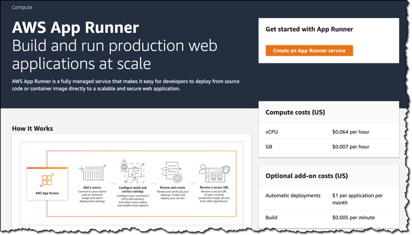
Introducing AWS App Runner
AWS App Runner makes it easier for you to deploy web apps and APIs to the cloud, regardless of the language they are written in, even for teams that lack prior experience deploying and managing containers or infrastructure. The service has AWS operational and security best practices built-it and automatically scale up or down at a moment’s notice, with no cold starts to worry about.

Deploying from Source
App Runner can deploy your app by either connecting to your source code or to a container registry. I will first show you how it works when connecting to source code. I have a Python web application in a GitHub repository. I will connect App Runner to this project, so you can see how it compiles and deploys my code to AWS.

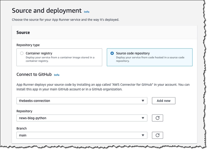
In the App Runner console, I choose Create an App Runner service.

Screenshot of the App Runner Console

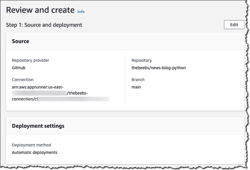
For Repository type, I choose Source code repository and then follow the instructions to connect the service to my GitHub account. For Repository, I choose the repository that contains the application I want to deploy. For Branch, I choose main.

Screenshot of source and deployment section of the console

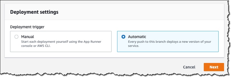
For Deployment trigger, I choose Automatic. This means when App Runner discovers a change to my source code, it automatically builds and deploys the updated version to my App Runner service

Screenshot of the deployment settings section of the console

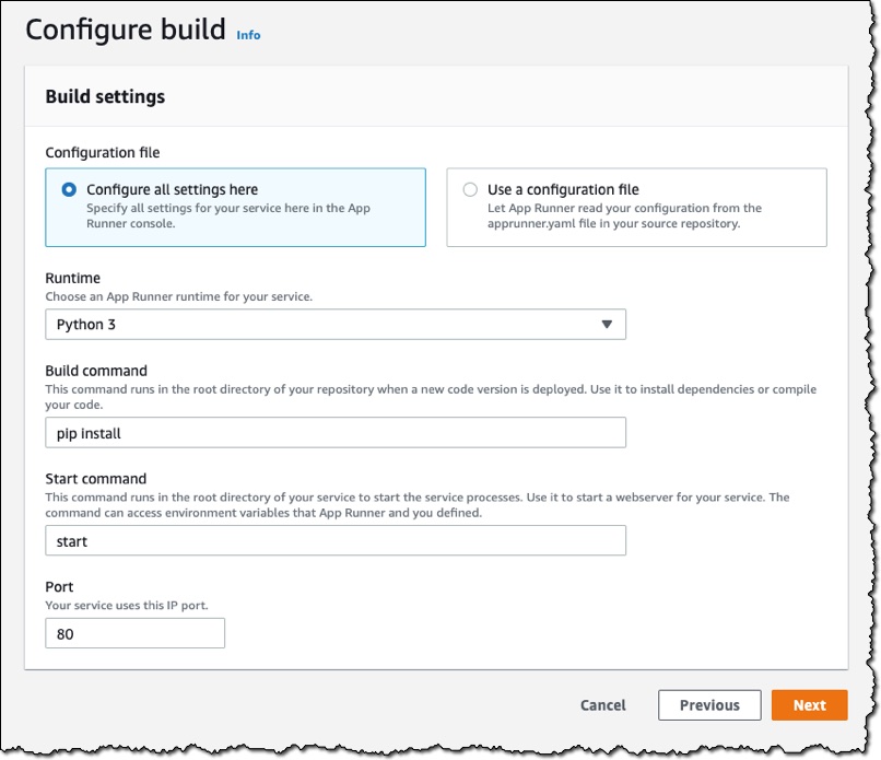
I can now configure the build. For Runtime, I choose Python 3. The service currently supports two languages: Python and Node.js. If you require other languages, then you will need to use the container registry workflow (which I will demonstrate later). I also complete the Build command, Start command, and Port fields, as shown here:

Screenshot of the Configure build section of the console

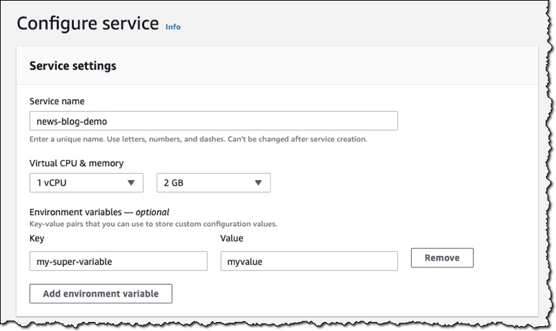
I now give my service a name and choose the CPU and memory size that I want my container to have. The choices I make here will affect the price I pay. Because my application requires very little CPU or memory, I choose 1 vCPU and 2 GB to keep my costs low. I can also provide any environment variables here to configure my application.

Screenshot of the configure service section of the console

The console allows me to customize several different settings for my service.

I can configure the auto scaling behavior. By default, my service will have one instance of my container image, but if the service receives more than 80 concurrent requests, it will scale to multiple instances. You can optionally specify a maximum number for cost control.

I can expand Health check, and set a path to which App Runner sends health check requests. If I do not set the path, App Runner attempts to make a TCP connection to verify health. By default, if App Runner receives five consecutive health check failures, it will consider the instance unhealthy and replace it.

I can expand Security, and choose an IAM role to be used by the instance. This will give permission for the container to communicate with other AWS services. App Runner encrypts all stored copies of my application source image or source bundle. If I provide a customer-managed key (CMK), App Runner uses it to encrypt my source. If I do not provide one, App Runner uses an AWS-managed key instead.

Screenshot of the console

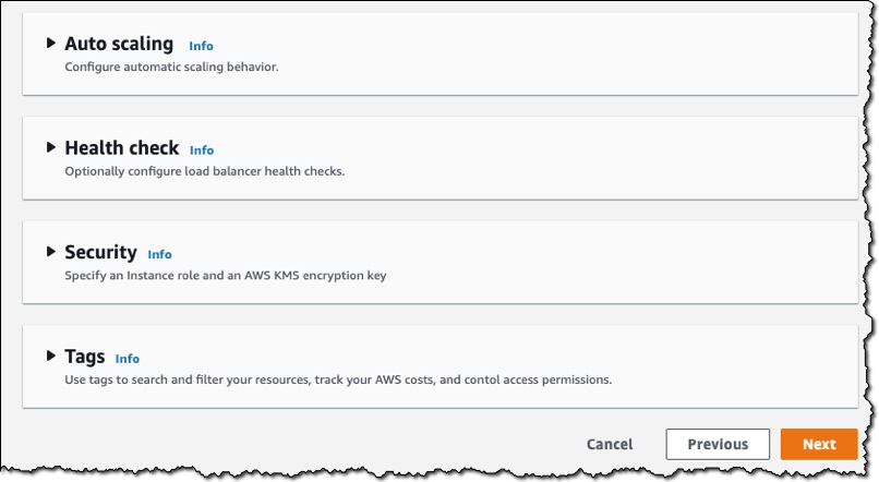
Finally, I review the configuration of the service and then choose Create & deploy.

Screenshot of the review and create section of the console

After a few minutes, my application was deployed and the service provided a URL that points to my deployed web application. App Runner ensures that https is configured so I can share it with someone on my team to test the application, without them receiving browser security warnings. I do not need to implement the handling of HTTPS secure traffic in my container image App Runner configures the whole thing.

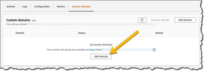
I now want to set up a custom domain. The service allows me to configure it without leaving the console. I open my service, choose the Custom domains tab, and then choose Add domain.

Screenshot of the custom domain section of the console

In Domain name, I enter the domain I want to use for my app, and then choose Save.

Screenshot of user adding a custom domain

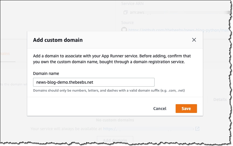
After I prove ownership of the domain, the app will be available at my custom URL. Next, I will show you how App Runner works with container images.

Deploy from a Container Image
I created a .NET web application, built it as a container image, and then pushed this container image to Amazon ECR Public (our public container registry).

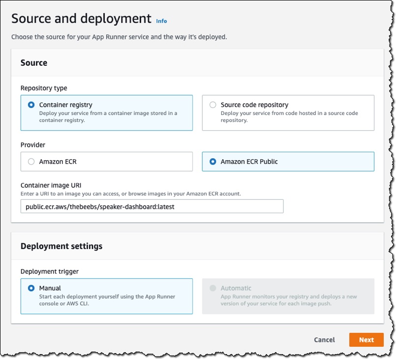
Just as I did in the first demo, I choose Create service. On Source and deployment, for Repository type, I choose Container registry. For Provider, I choose Amazon ECR Public. In Container image URI, I enter the URI to the image.

The deployment settings now only provide the option to manually trigger the deployment. This is because I chose Amazon ECR Public. If I wanted to deploy every time a container changed, then for Provider, I would need to choose Amazon ECR.

Screenshot of source and deployment section of the console

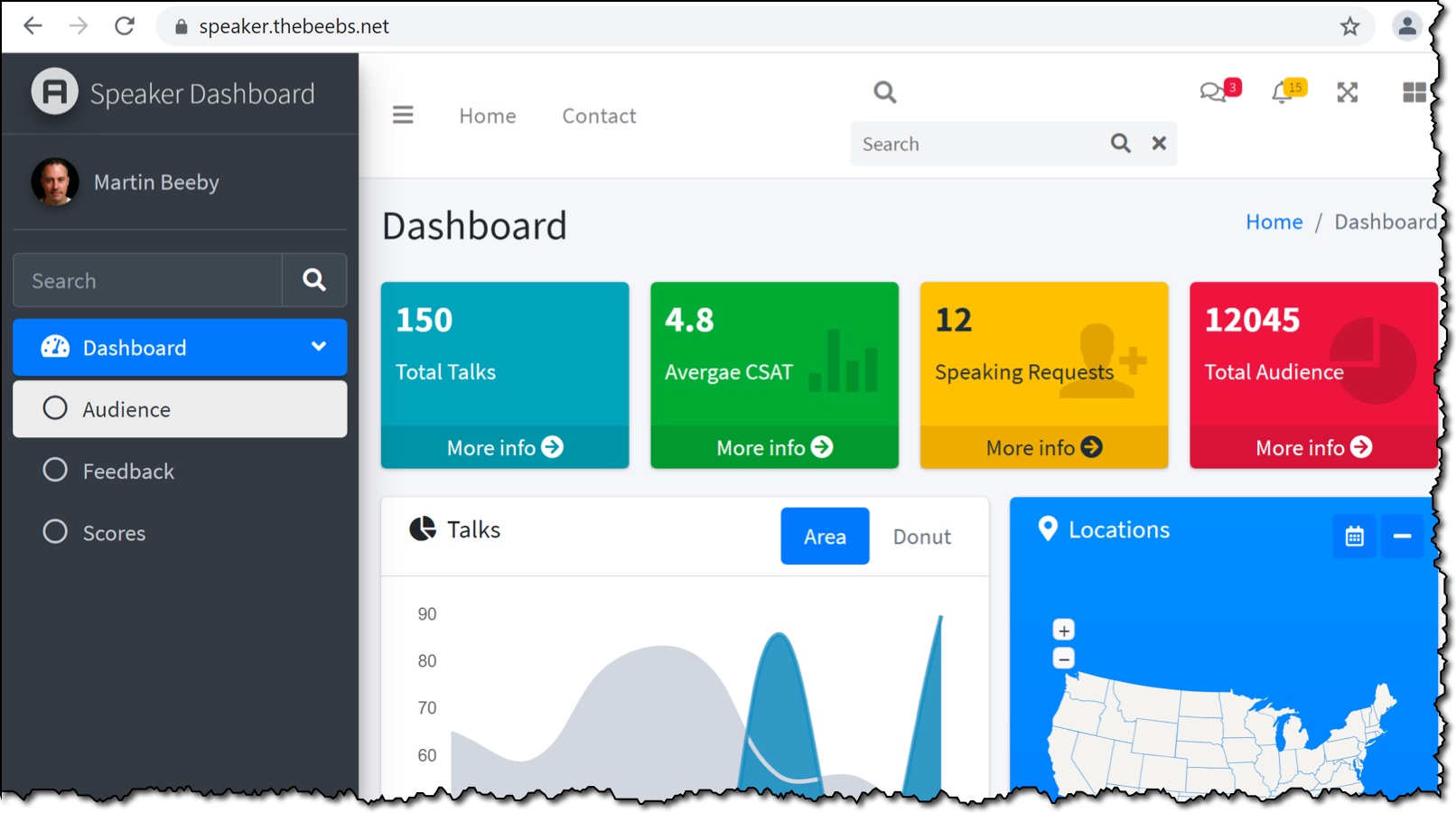
From this point on, the instructions are identical to those in the “Deploying from Source” section. After the deployment, the service provides a URL, and my application is live on the internet.

Screenshot of the app running

Things to Know
App Runner implements the file system in your container instance as ephemeral storage. Files are temporary. For example, they do not persist when you pause and resume your App Runner service. More generally, files are not guaranteed to persist beyond the processing of a single request, as part of the stateless nature of your application. Stored files do, however, take up part of the storage allocation of your App Runner service for the duration of their lifespan. Although ephemeral storage files are not guaranteed to persist across requests, they might sometimes persist. You can opportunistically take advantage of it. For example, when handling a request, you can cache files that your application downloads if future requests might need them. This might speed up future request handling, but I cannot guarantee the speed gains. Your code should not assume that a file that has been downloaded in a previous request still exists. For guaranteed caching, use a high-throughput, low-latency, in-memory data store like Amazon ElastiCache.

Partners in Action
We have been working with partners such as MongoDB, Datadog and HashiCorp to integrate with App Runner. Here is a flavor of what they have been working on:

MongoDB – “We’re excited to integrate App Runner with MongoDB Atlas so that developers can leverage the scalability and performance of our global, cloud-native database service for their App Runner applications.”

Datadog – “Using AWS App Runner, customers can now more easily deploy and scale their web applications from a container image or source code repository. With our new integration, customers can monitor their App Runner metrics, logs, and events to troubleshoot issues faster, and determine the best resource and scaling settings for their app.”

HashiCorp – “Integrating HashiCorp Terraform with AWS App Runner means developers have a faster, easier way to deploy production cloud applications, with less infrastructure to configure and manage.”

We also have exciting integrations from PulumiLogz.io, and Sysdig, which will allow App Runner customers to use the tools and service they already know and trust. As an AWS Consulting Partner, Trek10 can help customers leverage App Runner for cloud-native architecture design.

Availability and Pricing
AWS App Runner is available today in US East (N. Virginia), US West (Oregon), US East (Ohio), Asia Pacific (Tokyo), Europe (Ireland). You can use App Runner with the AWS Management Console and AWS Copilot CLI.

With App Runner, you pay for the compute and memory resources used by your application. App Runner automatically scales the number of active containers up and down to meet the processing requirements of your application. You can set a maximum limit on the number of containers your application uses so that costs do not exceed your budget.

You are only billed for App Runner when it is running and you can pause your application easily and resume it quickly. This is particularly useful in development and test situations as you can switch off an application when you are not using it, helping you manage your costs. For more information, see the App Runner pricing page.

Start using AWS App Runner today and run your web applications at scale, quickly and securely.

— Martin


Resolve IT Incidents Faster with Incident Manager, a New Capability of AWS Systems Manager

IT engineers pride themselves on the skill and care they put into building applications and infrastructure. However, as much as we all hate to admit it, there is no such thing as 100% uptime. Everything will fail at some point, often at the worst possible time, leading to many a ruined evening, birthday party, or wedding anniversary (ask me how I know).

As pagers go wild, on-duty engineers scramble to restore service, and every second counts. For example, you need to be able to quickly filter the deluge of monitoring alerts in order to pinpoint the root cause of the incident. Likewise, you can’t afford to waste any time locating and accessing the appropriate runbooks and procedures needed to solve the incident. Imagine yourself at 3:00A.M., wading in a sea of red alerts and desperately looking for the magic command that was “supposed to be in the doc.” Trust me, it’s not a pleasant feeling.

Serious issues often require escalations. Although it’s great to get help from team members, collaboration and a speedy resolution require efficient communication. Without it, uncoordinated efforts can lead to mishaps that confuse or worsen the situation.

Last but not least, it’s equally important to document the incident and how you responded to it. After the incident has been resolved and everyone has had a good night’s sleep, you can replay it, and work to continuously improve your platform and incident response procedures.

All this requires a lot of preparation based on industry best practices and appropriate tooling. Most companies and organizations simply cannot afford to learn this over the course of repeated incidents. That’s a very frustrating way to build an incident preparation and response practice.

Accordingly, many customers have asked us to help them, and today, I’m extremely happy to announce Incident Manager, a new capability of AWS Systems Manager that helps you prepare and respond efficiently to application and infrastructure incidents.

If you can’t wait to try it, please feel free to jump now to the Incident Manager console. If you’d like to learn more, read on!

Introducing Incident Manager in AWS Systems Manager
Since the launch of Amazon.com in 1995, Amazon teams have been responsible for incident response of their services. Over the years, they’ve accumulated a wealth of experience in responding to application and infrastructure issues at any scale. Distilling these years of experience, the Major Incident Management team at Amazon has designed Incident Manager to help all AWS customers prepare for and resolve incidents faster.

As preparation is key, Incident Manager lets you easily create a collection of incident response resources that are readily available when an alarm goes off. These resources include:

  • Contacts: Team members who may be engaged in solving incidents and how to page them (voice, email, SMS).
  • Escalation plans: Additional contacts who should be paged if the primary on-call responder doesn’t acknowledge the incident.
  • Response plans: Who to engage (contacts and escalation plan), what they should do (the runbook to follow), and where to collaborate (the channel tied to AWS Chatbot).

Incident Manager

In short, creating a response plan lets you prepare for incidents in a standardized way, so you can react as soon as they happen and resolve them quicker. Indeed, response plans can be triggered automatically by a Amazon CloudWatch alarm or an Amazon EventBridge event notification of your choice. If required, you can also launch a response plan manually.

When the response plan is initiated, contacts are paged, and a new dashboard is automatically put in place in the Incident Manager console. This dashboard is the point of reference for all things involved in the incident:

  • An overview on the incident, so that responders have a quick and accurate summary of the situation.
  • CloudWatch metrics and alarm graphs related to the incident.
  • A timeline of the incident that lists all events added by Incident Manager, and any custom event added manually by responders.
  • The runbook included in the response plan, and its current state of execution. Incident Manager provides a default template implementing triage, diagnosis, mitigation and recovery steps.
  • Contacts, and a link to the chat channel.
  • The list of related Systems Manager OpsItems.

Here’s a sample dashboard. As you can see, you can easily access all of the above in a single click.

Incident Dashboard

After the incident has been resolved, you can create a post-incident analysis, using a built-in template (based on the one that Amazon uses for Correction of Error), or one that you’ve created. This analysis will help you understand the root cause of the incident and what could have been done better or faster to resolve it.

By reviewing and editing the incident timeline, you can zoom in on specific events and how they were addressed. To guide you through the process, questions are automatically added to the analysis. Answering them will help you focus on potential improvements, and how to add them to your incident response procedures. Here’s a sample analysis, showing some of these questions.

Incident Analysis

Finally, Incident Manager recommends action items that you can accept or dismiss. If you accept an item, it’s added to a checklist that has to be fully completed before the analysis can be closed. The item is also filed as an OpsItem in AWS Systems Manager OpsCenter, which can sync to ticketing systems like Jira and ServiceNow.

Getting Started
The secret sauce in successfully responding to IT incidents is to prepare, prepare again, and then prepare some more. We encourage you to start planning now for failures that are waiting to happen. When that pager alarm comes in at 3:00AM, it will make a world of difference.

We believe Incident Manager will help you resolve incidents faster by improving your preparation, resolution and analysis workflows. It’s available today in the following AWS Regions:

  • US East (N. Virginia), US East (Ohio), US West (Oregon)
  • Europe (Ireland), Europe (Frankfurt), Europe (Stockholm)
  • Asia Pacific (Tokyo), Asia Pacific (Singapore), Asia Pacific (Sydney)

Give it a try, and let us know what you think. As always, we look forward to your feedback. You can send it through your usual AWS Support contacts, or post it on the AWS Forum for AWS Systems Manager.

If you want to learn more about Incident Manager, sign up for the AWS Summit Online event taking place on May 12 and 13, 2021.

New Amazon FinSpace Simplifies Data Management and Analytics for Financial Services

Managing data is the core of the Financial Services Industry (FSI). I worked for private banking and fund management companies and helped analysts to collect, aggregate, and analyze hundreds of petabytes of data from internal data sources, such as portfolio management, order management, and accounting systems, but also from external data sources, such as real-time market feeds and historical equities pricing and alternative data systems. During that period, I spent my time trying to access data across organizational silos, to manage permissions, and to build systems to automate recurring tasks in ever-growing and more complex environments.

Today, we are launching a solution that would have reduced the time I spent on such projects: Amazon FinSpace is a data management and analytics solution purpose-built for the financial services industry. Amazon FinSpace reduces the time it takes to find and prepare data from months to minutes so analysts can spend more time on analysis.

What Our Customers Told Us
Before data can be combined and analyzed, analysts spend weeks or months to find and access data across multiple departments, each specialized by market, instrument, or geography. In addition to this logical segregation, data is also physically isolated in different IT systems, file systems, or networks. Because access to data is strictly controlled by governance and policy, analysts must prepare and explain access requests to the compliance department. This is a very manual, ad-hoc process.

Once granted access, they often must perform computational logic (such as Bollinger Bands, Exponential Moving Average, or Average True Range) on larger and larger datasets to prepare data for analysis or to derive information out of the data. These computations often run on servers with constrained capacity, as they were not designed to handle the size of workloads in the modern financial world. Even server-side systems are struggling to scale up and keep up with the ever-growing size of the datasets they need to store and analyze.

How Amazon FinSpace Helps
Amazon FinSpace removes the undifferentiated heavy lifting required to store, prepare, manage, and audit access to data. It automates the steps involved in finding data and preparing it for analysis. Amazon FinSpace stores and organizes data using industry and internal data classification conventions. Analysts connect to the Amazon FinSpace web interface to search for data using familiar business terms (“S&P500,” “CAC40,” “private equity funds in euro”).

Analysts can prepare their chosen datasets using a built-in library of more than 100 specialized functions for time series data. They can use the integrated Jupyter notebooks to experiment with data, and parallelize these financial data transformations at the scale of the cloud in minutes. Finally, Amazon FinSpace provides a framework to manage data access and to audit who is accessing what data and when. It tracks usage of data and generates compliance and audit reports.

Amazon FinSpace also makes it easy to work on historical data. Let’s imagine I built a model to calculate credit risk. This model relies on interest rate and inflation rate. These two rates get updated frequently. The risk level associated with a customer is not the same today as it was a few months ago, when inflation and interest rates were different. When data analysts are looking at data as it is now and as it was in the past, they call it bitemporal modeling. Amazon FinSpace makes it easy to go back in time and to compare how models are evolving alongside multiple dimensions.

To show you how Amazon FinSpace works, let’s imagine I have a team of analysts and data scientists and I want to provide them a tool to search, prepare, and analyze data.

How to Create an Amazon FinSpace Environment
As an AWS account administrator, I create a working environment for my team of financial analysts. This is a one-time setup.

I navigate to the Amazon FinSpace console and click Create Environment:

FinSpace Create environment

I give my environment a name. I select a KMS encryption key that will serve to encrypt data at rest. Then I choose either to integrate with AWS Single Sign-On or to manage usernames and passwords in Amazon FinSpace. AWS Single Sign-On integration allows your analysts to authenticate with external systems, such as a corporate Active Directory, to access the Amazon FinSpace environment. For this example, I choose to manage the credentials by myself.

FinSpace create environment details

I create a superuser who will have administration permission on the Amazon FinSpace environment. I click Add Superuser:

Finspace create super user 1Finspace create super user 2I take a note of the temporary password. I copy the text of the message to send to my superuser. This message includes the connection instructions for the initial connection to the environment.

The superuser has permission to add other users and to manage these users’ permissions in the Amazon FinSpace environment itself.

Finally, and just for the purpose of this demo, I choose to import an initial dataset. This allows me to start with some data in the environment. Doing so is just a single click in the console. The storage cost of this dataset is $41.46 / month and I can delete it at any time.

Under Sample data bundles, Capital Markets sample data, I click Install dataset. This can take several minutes, so it’s a good time to stand up, stretch your legs, and grab a cup of coffee.

FinSpace install sample dataset

How to Use an Amazon FinSpace Environment
In my role as financial analyst, my AWS account administrator sends me an email containing a URL to connect to my Amazon FinSpace Environment along with the related credentials. I connect to the Amazon FinSpace environment.

A couple of points are worth noting on the welcome page. First, on the top right side, I click the gear icon to access the environment settings. This is where I can add other users and manage their permissions. Second, you can browse the different data by categories on the left side, or search for specific terms by typing your search query on the search bar on top of the screen, and refine your search on the left side.

I can use Amazon FinSpace as my data hub. Data are fed through the API or I can load data directly from my workstation. I use tags to describe datasets. Datasets are containers for data; changes are versioned and I can create historical views of data or use the auto-updating data view that Amazon FinSpace maintains for me.

For this demo, let’s imagine I received a request from a portfolio manager who wants a chart showing realized volatility using 5 minute time bars for AMZN stock. Let me show you how I use the search bar to locate data and then use a notebook to analyze that data.

First, I search my dataset for stock price time bar summary, with 5 min intervals. I type “equity” in the search box. I’m lucky: The first result is the one I want. If needed, I could have refined the results using the facets on the left.

finspace search equity

Once I find the dataset, I explore its description, the schema, and other information. Based on these, I decide if this is the correct dataset to answer my portfolio manager’s request.

finspace dataset details


I click Analyze in notebook to start a Jupyter notebook where I’ll be able to further explore the data with PySpark. Once the notebook is open, I first check it is correctly configured to use the Amazon FinSpace PySpark kernel (starting the kernel takes 5-8 minutes).

Finspace select kernel

I click “play” on the first code box to connect to the Spark cluster.

finspace connect to cluster

To analyze my dataset and answer the specific question from my PM, I need to type a bit of PySpark code. For the purpose of this demo, I am using sample code from the Amazon FinSpace GitHub repository. You can upload the Notebook to your environment. Click the up arrow as shown on the top left of the screen above to select the file from your local machine.

This notebook pulls data from the Amazon FinSpace catalog “US Equity Time-Bar Summary” data I found earlier, and then uses the Amazon FinSpace built-in analytic function realized_volatility() to compute realized volatility for a group of tickers and exchange event types.

Before creating any graph, let’s have a sense of the dataset. What is the time range of the data ? What tickers are in this dataset ? I answer these questions with simple select() or groupby() functions provided by Amazon FinSpace. I prepare my FinSpaceAnalyticsAnalyser class with the code below :

from aws.finspace.analytics import FinSpaceAnalyticsManager
finspace = FinSpaceAnalyticsManager(spark = spark, endpoint=hfs_endpoint)

sumDF = finspace.read_data_view(dataset_id = dataset_id, data_view_id = view_id)

Once done, I can start to explore the dataset:
finspace analysis 1

I can see there are 561778 AMZN trades and price quotes between Oct. 1, 2019 and March 31, 2020.

To plot the realized volatility, I use Panda to plot the values:

finspace plot realized volatility code

When I execute this code block, I receive:

finspace plot realized volatility graph


Similarly, I can start a Bollinger Bands analysis to check if the volatility spike created an oversold condition on the AMZN stock. I am also using Panda to plot the values.

finspace plot bollinger bandcode

and generate this graph:

finspace plot realized volatility bolinger graph


I am ready to answer the portfolio manager’s question. But why was there a spike on Jan 30 2020 ? The answer is in the news: “Amazon soars after huge earnings beat.” 🙂

Availability and Pricing
Amazon FinSpace is available today in US East (N. Virginia), US East (Ohio), US West (Oregon), Europe (Ireland), and Canada (Central).

As usual, we charge you only for the resources your project uses. Pricing is based on three dimensions: the number of analysts with access to the service, the volume of data ingested, and the compute hours used to apply your transformations. Detailed pricing information is available on the service pricing page.

Give it a try today and let us know your feedback.

— seb

Introducing CloudFront Functions – Run Your Code at the Edge with Low Latency at Any Scale

With Amazon CloudFront, you can securely deliver data, videos, applications, and APIs to your customers globally with low latency and high transfer speeds. To offer a customized experience and the lowest possible latency, many modern applications execute some form of logic at the edge. The use cases for applying logic at the edge can be grouped together in two main categories:

  • First are the complex, compute-heavy operations that are executed when objects are not in the cache. We launched Lambda@Edge in 2017 to offer a fully programmable, serverless edge computing environment for implementing a wide variety of complex customizations. Lambda@Edge functions are executed in a regional edge cache (usually in the AWS region closest to the CloudFront edge location reached by the client). For example, when you’re streaming video or audio, you can use Lambda@Edge to create and serve the right segments on-the-fly reducing the need for origin scalability. Another common use case is to use Lambda@Edge and Amazon DynamoDB to translate shortened, user-friendly URLs to full URL landing pages.
  • The second category of use cases are simple HTTP(s) request/response manipulations that can be executed by very short-lived functions. For these use cases, you need a flexible programming experience with the performance, scale, and cost-effectiveness that enable you to execute them on every request.

To help you with this second category of use cases, I am happy to announce the availability of CloudFront Functions, a new serverless scripting platform that allows you to run lightweight JavaScript code at the 218+ CloudFront edge locations at approximately 1/6th the price of Lambda@Edge.

Architectural diagram.

CloudFront Functions are ideal for lightweight processing of web requests, for example:

  • Cache-key manipulations and normalization: Transform HTTP request attributes (such as URL, headers, cookies, and query strings) to construct the cache-key, which is the unique identifier for objects in cache and is used to determine whether an object is already cached. For example, you could cache based on a header that contains the end user’s device type, creating two different versions of the content for mobile and desktop users. By transforming the request attributes, you can also normalize multiple requests to a single cache-key entry and significantly improve your cache-hit ratio.
  • URL rewrites and redirects: Generate a response to redirect requests to a different URL. For example, redirect a non-authenticated user from a restricted page to a login form. URL rewrites can also be used for A/B testing.
  • HTTP header manipulation: View, add, modify, or delete any of the request/response headers. For instance, add HTTP Strict Transport Security (HSTS) headers to your response, or copy the client IP address into a new HTTP header so that it is forwarded to the origin with the request.
  • Access authorization: Implement access control and authorization for the content delivered through CloudFront by creating and validating user-generated tokens, such as HMAC tokens or JSON web tokens (JWT), to allow/deny requests.

To give you the performance and scale that modern applications require, CloudFront Functions uses a new process-based isolation model instead of virtual machine (VM)-based isolation as used by AWS Lambda and Lambda@Edge. To do that, we had to enforce some restrictions, such as avoiding network and file system access. Also, functions run for less than one millisecond. In this way, they can handle millions of requests per second while giving you great performance on every function execution. Functions add almost no perceptible impact to overall content delivery network (CDN) performance.

Similar to Lambda@Edge, CloudFront Functions runs your code in response to events generated by CloudFront. More specifically, CloudFront Functions can be triggered after CloudFront receives a request from a viewer (viewer request) and before CloudFront forwards the response to the viewer (viewer response).

Lambda@Edge can also be triggered before CloudFront forwards the request to the origin (origin request) and after CloudFront receives the response from the origin (origin response). You can use CloudFront Functions and Lambda@Edge together, depending on whether you need to manipulate content before, or after, being cached.

Architectural diagram.

If you need some of the capabilities of Lambda@Edge that are not available with CloudFront Functions, such as network access or a longer execution time, you can still use Lambda@Edge before and after content is cached by CloudFront.

Architectural diagram.

To help you understand the difference between CloudFront Functions and Lambda@Edge, here’s a quick comparison:

CloudFront Functions Lambda@Edge
Runtime support JavaScript
(ECMAScript 5.1 compliant)
Node.js, Python
Execution location 218+ CloudFront
Edge Locations
13 CloudFront
Regional Edge Caches
CloudFront triggers supported Viewer request
Viewer response
Viewer request
Viewer response
Origin request
Origin response
Maximum execution time Less than 1 millisecond 5 seconds (viewer triggers)
30 seconds (origin triggers)
Maximum memory 2MB 128MB (viewer triggers)
10GB (origin triggers)
Total package size 10 KB 1 MB (viewer triggers)
50 MB (origin triggers)
Network access No Yes
File system access No Yes
Access to the request body No Yes
Pricing Free tier available;
charged per request
No free tier; charged per request
and function duration

Let’s see how this works in practice.

Using CloudFront Functions From the Console
I want to customize the content of my website depending on the country of origin of the viewers. To do so, I use a CloudFront distribution that I created using an S3 bucket as origin. Then, I create a cache policy to include the CloudFront-Viewer-Country header (that contains the two-letter country code of the viewer’s country) in the cache key. CloudFront Functions can see CloudFront-generated headers (like the CloudFront geolocation or device detection headers) only if they are included in an origin policy or cache key policy.

In the CloudFront console, I select Functions on the left bar and then Create function. I give the function a name and Continue.

Console screenshot.

From here, I can follow the lifecycle of my function with these steps:

  1. Build the function by providing the code.
  2. Test the function with a sample payload.
  3. Publish the function from the development stage to the live stage.
  4. Associate the function with one or more CloudFront distributions.

Console screenshot.

1. In the Build tab, I can access two stages for each function: a Development stage for tests, and a Live stage that can be used by one or more CloudFront distributions. With the development stage selected, I type the code of my function and Save:

function handler(event) {
  var request = event.request;
  var supported_countries = ['de', 'it', 'fr'];
  if (request.uri.substr(3,1) != '/') {
    var headers = request.headers;
    var newUri;
    if (headers['cloudfront-viewer-country']) {
      var countryCode = headers['cloudfront-viewer-country'].value.toLowerCase();
      if (supported_countries.includes(countryCode)) {
        newUri = '/' + countryCode + request.uri;
      }
    }
    if (newUri === undefined) {
      var defaultCountryCode = 'en';
      newUri = '/' + defaultCountryCode + request.uri;
    }
    var response = {
      statusCode: 302,
      statusDescription: 'Found',
      headers: {
        "location": { "value": newUri }
      }
    }
    return response;
  }
  return request;
}

The function looks at the content of the CloudFront-Viewer-Country header set by CloudFront. If it contains one of the supported countries, and the URL does not already contain a country prefix, it adds the country at the beginning of the URL path. Otherwise, it lets the request pass through without changes.

2. In the Test tab, I select the event type (Viewer Request), the Stage (Development, for now) and a sample event.

Console screenshot.

Below, I can customize the Input event by selecting the HTTP method, and then editing the path of the URL, and optionally the client IP to use. I can also add custom headers, cookies, or query strings. In my case, I leave all the default values and add the CloudFront-Viewer-Country header with the value of FR (for France). Optionally, instead of using the visual editor, I can customize the input event by editing the JSON payload that is passed to the function.

Console screenshot.

I click on the Test button and look at the Output. As expected, the request is being redirected (HTTP status code 302). In the Response headers, I see that the location where the request is being redirected starts with /fr/ to provide custom content for viewers based in France. If something doesn’t go as expected in my tests, I can look at the Function Logs. I can also use console.log() in my code to add more debugging information.

Console screenshot.

In the Output, just above the HTTP status, I see the Compute utilization for this execution. Compute utilization is a number between 0 and 100 that indicates the amount of time that the function took to run as a percentage of the maximum allowed time. In my case, a compute utilization of 21 means that the function completed in 21% of the maximum allowed time.

3. I run more tests using different configurations of URL and headers, then I move to the Publish tab to copy the function from the development stage to the live stage. Now, the function is ready to be associated with an existing distribution.

Console screenshot.

4. In the Associate tab, I select the Distribution, the Event type (Viewer Request or Viewer Response) and the Cache behavior (I only have the Default (*) cache behavior for my distribution). I click Add association and confirm in the dialog.

Console screenshot.

Now, I see the function association at the bottom of the Associate tab.

Console screenshot.

To test this configuration from two different locations, I start two Amazon Elastic Compute Cloud (Amazon EC2) instances, one in the US East (N. Virginia) Region and one in the Europe (Paris) Region. I connect using SSH and use cURL to get an object from the CloudFront distribution. Previously, I have uploaded two objects to the S3 bucket that is used as the origin for the distribution: one, for customers based in France, using the fr/ prefix, and one, for customers not in a supported country, using the en/ prefix.

I list the two objects using the AWS Command Line Interface (CLI):

$ aws s3 ls --recursive s3://BUCKET
2021-04-01 13:54:20         13 en/doc.txt
2021-04-01 13:54:20          8 fr/doc.txt

In the EC2 instance in the US East (N. Virginia) Region, I run this command to download the object:

[us-east-1]$ curl -L https://d2wj2l15gt32vo.cloudfront.net/doc.txt 
Good morning

Then I run the same command in the Europe (Paris) Region:

[eu-west-3]$ curl -L https://d2wj2l15gt32vo.cloudfront.net/doc.txt
Bonjour

As expected, I am getting different results from the same URL. I am using the -L option so that cURL is following the redirect it receives. In this way, each command is executing two HTTP requests: the first request receives the HTTP redirect from the CloudFront function, the second request follows the redirect and is not modified by the function because it contains a custom path in the URL (/en/ or /fr/).

To see the actual location of the redirect and all HTTP response headers, I use cURL with the -i option. These are the response headers for the EC2 instance running in the US; the function is executed at an edge location in Virginia:

[us-east-1]$ curl -i https://d2wj2l15gt32vo.cloudfront.net/doc.txt 
HTTP/2 302 
server: CloudFront
date: Thu, 01 Apr 2021 14:39:31 GMT
content-length: 0
location: /en/doc.txt
x-cache: FunctionGeneratedResponse from cloudfront
via: 1.1 cb0868a0a661911b98247aaff77bc898.cloudfront.net (CloudFront)
x-amz-cf-pop: IAD50-C2
x-amz-cf-id: TuaLKKg3YvLKN85fzd2qfcx9jOlfMQrWazpOVmN7NgfmmcXc1wzjmA==

And these are the response headers for the EC2 instance running in France; this time, the function is executed in an edge location near Paris:

[eu-west-3]$ curl -i https://d2wj2l15gt32vo.cloudfront.net/doc.txt
HTTP/2 302 
server: CloudFront
date: Thu, 01 Apr 2021 14:39:26 GMT
content-length: 0
location: /fr/doc.txt
x-cache: FunctionGeneratedResponse from cloudfront
via: 1.1 6fa25eadb94abd73b5efc56a89b2d829.cloudfront.net (CloudFront)
x-amz-cf-pop: CDG53-C1
x-amz-cf-id: jzWcbccJiTDRj22TGwsn_

Availability and Pricing
CloudFront Functions is available today and you can use it with new and existing distributions. You can use CloudFront Functions with the AWS Management Console, AWS Command Line Interface (CLI), AWS SDKs, and AWS CloudFormation. With CloudFront Functions, you pay by the number of invocations. You can get started with CloudFront Functions for free as part of the AWS Free Usage Tier. For more information, please see the CloudFront pricing page.

AWS for the Edge
Amazon CloudFront and AWS edge networking capabilities are part of the AWS for the Edge portfolio. AWS edge services improve performance by moving compute, data processing, and storage closer to end-user devices. This includes deploying AWS managed services, APIs, and tools to locations outside AWS data centers, and even onto customer-owned infrastructure and devices.

AWS offers you a consistent experience and portfolio of capabilities from the edge to the cloud. Using AWS, you have access to the broadest and deepest capabilities for edge use cases, like edge networking, hybrid architectures, connected devices, 5G, and multi-access edge computing.

Start using CloudFront Functions today to add custom logic at the edge for your applications.

Danilo